7.9. Determination of polarization

This notebook has a zz. prefix, because it has to be executed after the polarimeter fields are exported in Uncertainties.

Import Python libraries Hide code cell content

from __future__ import annotations

import itertools
import json
import logging
import os
from functools import lru_cache
from textwrap import dedent, wrap
from warnings import filterwarnings

import iminuit
import jax
import jax.numpy as jnp
import matplotlib.pyplot as plt
import numpy as np
import plotly.graph_objects as go
import yaml
from IPython.display import Latex, Markdown, display
from numpy import pi as π
from plotly.subplots import make_subplots
from scipy.interpolate import interp2d
from tensorwaves.interface import DataSample
from tqdm.auto import tqdm

from polarimetry.data import generate_phasespace_sample
from polarimetry.io import import_polarimetry_field, mute_jax_warnings
from polarimetry.lhcb import load_model_builder
from polarimetry.lhcb.particle import load_particles
from polarimetry.plot import use_mpl_latex_fonts

filterwarnings("ignore")
mute_jax_warnings()
logging.getLogger("tensorwaves.data").setLevel(logging.ERROR)

NO_TQDM = "EXECUTE_NB" in os.environ
if NO_TQDM:
    logging.getLogger().setLevel(logging.ERROR)
    logging.getLogger("polarimetry.io").setLevel(logging.ERROR)

Given the aligned polarimeter field \(\vec\alpha\) and the corresponding intensity distribution \(I_0\), the intensity distribution \(I\) for a polarized decay can be computed as follows:

(7.1)\[ I\left(\phi,\theta,\chi; \tau\right) = I_0(\tau)\left(1+\vec{P} R(\phi,\theta,\chi) \vec{\alpha}(\tau)\right) \]

with \(R\) the rotation matrix over the decay plane orientation, represented in Euler angles \(\left(\phi, \theta, \chi\right)\).

In this section, we show that it’s possible to determine the polarization \(\vec{P}\) from a given intensity distribution \(I\) of a \(\lambda_c\) decay if we the \(\vec\alpha\) fields and the corresponding \(I_0\) values of that \(\Lambda_c\) decay. We get \(\vec\alpha\) and \(I_0\) by interpolating the grid samples provided from Exported distributions using the method described in Import and interpolate. We perform the same procedure with the averaged aligned polarimeter vector from Section 5.6 in order to quantify the loss in precision when integrating over the Dalitz plane variables \(\tau\).

7.9.1. Polarized test distribution

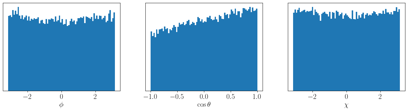
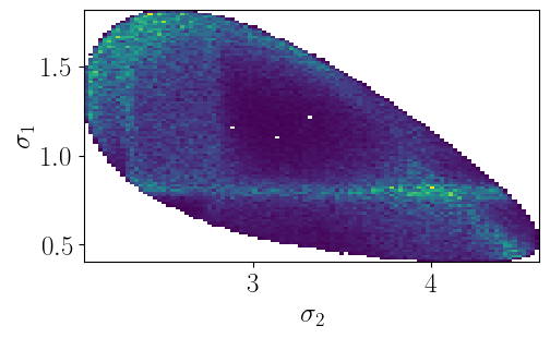
For this study, a phase space sample is uniformly generated over the Dalitz plane variables \(\tau\). The phase space sample is extended with uniform distributions over the decay plane angles \(\left(\phi, \theta, \chi\right)\), so that the phase space can be used to generate a hit-and-miss toy sample for a polarized intensity distribution.

Generate phase space sample Hide code cell source

DECAY = load_model_builder(
    "../data/model-definitions.yaml",
    load_particles("../data/particle-definitions.yaml"),
    model_id=0,
).decay

N_EVENTS = 100_000
# Dalitz variables
PHSP = generate_phasespace_sample(DECAY, N_EVENTS, seed=0)
# Decay plane variables
RNG = np.random.default_rng(seed=0)
PHSP["phi"] = RNG.uniform(-π, +π, N_EVENTS)
PHSP["cos_theta"] = RNG.uniform(-1, +1, N_EVENTS)
PHSP["chi"] = RNG.uniform(-π, +π, N_EVENTS)

We now generate an intensity distribution over the phase space sample given a certain value for \(\vec{P}\) [1] using Eq. (7.1) and by interpolating the \(\vec\alpha\) and \(I_0\) fields with the grid samples for the nominal model.

Code for interpolating α and I₀ Hide code cell source

def interpolate_intensity(phsp: DataSample, model_id: int) -> jax.Array:
    x = PHSP["sigma1"]
    y = PHSP["sigma2"]
    return jnp.array(create_interpolated_function(model_id, "intensity")(x, y))


def interpolate_polarimetry_field(phsp: DataSample, model_id: int) -> jax.Array:
    x = PHSP["sigma1"]
    y = PHSP["sigma2"]
    return jnp.array(
        [create_interpolated_function(model_id, f"alpha_{i}")(x, y) for i in "xyz"]
    )


@lru_cache(maxsize=0)
def create_interpolated_function(model_id: int, variable: str):
    field_file = f"_static/export/polarimetry-field-model-{model_id}.json"
    field_data = import_polarimetry_field(field_file)
    interpolated_func = interp2d(
        x=field_data["m^2_Kpi"],
        y=field_data["m^2_pK"],
        z=np.nan_to_num(field_data[variable]),
        kind="linear",
    )
    return np.vectorize(interpolated_func)

Code for computing polarized intensity Hide code cell source

def compute_polarized_intensity(
    Px: float,
    Py: float,
    Pz: float,
    I0: jax.Array,
    alpha: jax.Array,
    phsp: DataSample,
) -> jnp.array:
    P = jnp.array([Px, Py, Pz])
    R = compute_rotation_matrix(phsp)
    return I0 * (1 + jnp.einsum("i,ij...,j...->...", P, R, alpha))


def compute_rotation_matrix(phsp: DataSample) -> jax.Array:
    ϕ = phsp["phi"]
    θ = jnp.arccos(phsp["cos_theta"])
    χ = phsp["chi"]
    return jnp.einsum("ki...,ij...,j...->k...", Rz(ϕ), Ry(θ), Rz(χ))


def Rz(angle: jax.Array) -> jax.Array:
    n_events = len(angle)
    ones = jnp.ones(n_events)
    zeros = jnp.zeros(n_events)
    return jnp.array(
        [
            [+jnp.cos(angle), -jnp.sin(angle), zeros],
            [+jnp.sin(angle), +jnp.cos(angle), zeros],
            [zeros, zeros, ones],
        ]
    )


def Ry(angle: jax.Array) -> jax.Array:
    n_events = len(angle)
    ones = jnp.ones(n_events)
    zeros = jnp.zeros(n_events)
    return jnp.array(
        [
            [+jnp.cos(angle), zeros, +jnp.sin(angle)],
            [zeros, ones, zeros],
            [-jnp.sin(angle), zeros, +jnp.cos(angle)],
        ]
    )

P = (+0.2165, +0.0108, -0.665)
I = compute_polarized_intensity(
    *P,
    I0=interpolate_intensity(PHSP, model_id=0),
    alpha=interpolate_polarimetry_field(PHSP, model_id=0),
    phsp=PHSP,
)
I /= jnp.mean(I)  # normalized times N for log likelihood

Show code cell source Hide code cell source

plt.rc("font", size=18)
use_mpl_latex_fonts()

fig, axes = plt.subplots(figsize=(15, 4), ncols=3)
fig.tight_layout()
for ax in axes:
    ax.set_yticks([])
axes[0].hist(PHSP["phi"], weights=I, bins=80)
axes[1].hist(PHSP["cos_theta"], weights=I, bins=80)
axes[2].hist(PHSP["chi"], weights=I, bins=80)
axes[0].set_xlabel(R"$\phi$")
axes[1].set_xlabel(R"$\cos\theta$")
axes[2].set_xlabel(R"$\chi$")
plt.show()

fig, ax = plt.subplots(figsize=(12, 3))
ax.hist2d(PHSP["sigma2"], PHSP["sigma1"], weights=I, bins=100, cmin=1)
ax.set_xlabel(R"$\sigma_2$")
ax.set_ylabel(R"$\sigma_1$")
ax.set_aspect("equal")
plt.show()

7.9.2. Using the exported polarimeter grid

The generated distribution is now assumed to be a measured distribution \(I\) with unknown polarization \(\vec{P}\). It is shown below that the actual \(\vec{P}\) with which the distribution was generated can be found by performing a fit on Eq. (7.1). This is done with iminuit, starting with a certain ‘guessed’ value for \(\vec{P}\) as initial parameters.

To avoid having to generate a hit-and-miss intensity test distribution, the parameters \(\vec{P} = \left(P_x, P_y, P_z\right)\) are optimized with regard to a weighted negative log likelihood estimator:

(7.2)\[ \mathrm{NLL} = -\sum_i w_i \log I_{i,\vec{P}}\left(\phi,\theta,\chi;\tau\right)\,. \]

with the normalized intensities of the generated distribution taken as weights:

(7.3)\[ w_i = n\,I_i\,\big/\,\sum_j^n I_j\,, \]

such that \(\sum w_i = n\). To propagate uncertainties, a fit is performed using the exported grids of each alternative model.

P_GUESS = (+0.3, -0.3, +0.4)

Fit polarization with full polarimeter field Hide code cell source

def perform_field_fit(phsp: DataSample, model_id: int) -> iminuit.Minuit:
    I0 = interpolate_intensity(phsp, model_id)
    alpha = interpolate_polarimetry_field(phsp, model_id)

    def weighted_nll(Px: float, Py: float, Pz: float) -> float:
        I_new = compute_polarized_intensity(Px, Py, Pz, I0, alpha, phsp)
        I_new /= jnp.sum(I_new)
        return -jnp.sum(jnp.log(I_new) * I)

    optimizer = iminuit.Minuit(weighted_nll, *P_GUESS)
    optimizer.errordef = optimizer.LIKELIHOOD
    return optimizer.migrad()


SYST_FIT_RESULTS_FIELD = [
    perform_field_fit(PHSP, i)
    for i in tqdm(range(18), desc="Performing fits", disable=NO_TQDM)
]

Show Minuit fit result for nominal model Hide code cell content

SYST_FIT_RESULTS_FIELD[0]

Migrad
FCN = 1.127e+06	Nfcn = 66
EDM = 2.58e-06 (Goal: 0.0001)	time = 3.2 sec
Valid Minimum	Below EDM threshold (goal x 10)
No parameters at limit	Below call limit
Hesse ok	Covariance accurate

	Name	Value	Hesse Error	Minos Error-	Minos Error+	Limit-	Limit+	Fixed
0	Px	0.217	0.008
1	Py	0.011	0.008
2	Pz	-0.665	0.007

	Px	Py	Pz
Px	6.24e-05	0	0 (0.042)
Py	0	6.27e-05	0
Pz	0 (0.042)	0	5.6e-05

Show code cell source Hide code cell source

def extract_polarizations(fit_results: list[iminuit.Minuit]) -> np.ndarray:
    return np.array([extract_polarization(fit) for fit in fit_results])


def extract_polarization(fit_result: iminuit.Minuit) -> tuple[float, float, float]:
    return tuple(p.value for p in fit_result.params)


def render_fit_results(
    fit_results: list[iminuit.Minuit],
    compare: bool = False,
) -> str:
    P_syst = 100 * extract_polarizations(fit_results)
    P_nominal = P_syst[0]
    P_max = (P_syst[1:] - P_nominal).max(axis=0)
    P_min = (P_syst[1:] - P_nominal).min(axis=0)
    if compare:
        np.testing.assert_array_almost_equal(P_nominal, 100 * np.array(P), decimal=2)

    def render_p(i: int) -> str:
        return f"{P_nominal[i]:+.2f}_{{{P_min[i]:+.2f}}}^{{{P_max[i]:+.2f}}}"

    src = Rf"""
    \begin{{array}}{{ccc}}
    P_x &=& {render_p(0)} \\
    P_y &=& {render_p(1)} \\
    P_z &=& {render_p(2)} \\
    \end{{array}}
    """
    return dedent(src).strip()


src = Rf"""
The polarization $\vec{{P}}$ is determined to be (in %):

$$
{render_fit_results(SYST_FIT_RESULTS_FIELD, compare=True)}
$$

with the upper and lower sign being the systematic extrema uncertainties as determined by
the alternative models.
"""
Markdown(src)

The polarization \(\vec{P}\) is determined to be (in %):

\[\begin{split} \begin{array}{ccc} P_x &=& +21.65_{-0.62}^{+0.30} \\ P_y &=& +1.08_{-0.05}^{+0.02} \\ P_z &=& -66.50_{-0.85}^{+1.66} \\ \end{array} \end{split}\]

with the upper and lower sign being the systematic extrema uncertainties as determined by the alternative models.

This is to be compared with the model uncertainties reported by [1]:

\[\begin{split} \begin{array}{ccc} P_x &=& +21.65 \pm 0.36 \\ P_y &=& +1.08 \pm 0.09 \\ P_z &=& -66.5 \pm 1.1. \\ \end{array} \end{split}\]

The polarimeter values for each model are (in %):

Show code cell source Hide code cell source

def render_all_polarizations(fit_results: list[iminuit.Minuit]) -> Latex:
    src = R"""
    \begin{array}{r|ccc|ccc}
      \textbf{Model} & \mathbf{P_x} & \mathbf{P_y} & \mathbf{P_z}
      & \mathbf{\Delta P_x} & \mathbf{\Delta P_y} & \mathbf{\Delta P_z} \\
      \hline
    """
    P_fit_values = np.array([extract_polarization(fit) for fit in fit_results])
    P_fit_values *= 100
    Px_nom, Py_nom, Pz_nom = P_fit_values[0]
    for i, (Px, Py, Pz) in enumerate(P_fit_values):
        src += Rf"  \textbf{{{i}}} & {Px:+.2f} & {Py:+.2f} & {Pz:+.1f} & "
        if i != 0:
            src += Rf"{Px-Px_nom:+.2f} & {Py-Py_nom:+.2f} & {Pz-Pz_nom:+.2f}"
        src += R" \\" "\n"
    src += R"\end{array}"
    src = dedent(src).strip()
    return Latex(src)


render_all_polarizations(SYST_FIT_RESULTS_FIELD)

\[\begin{split}\begin{array}{r|ccc|ccc} \textbf{Model} & \mathbf{P_x} & \mathbf{P_y} & \mathbf{P_z} & \mathbf{\Delta P_x} & \mathbf{\Delta P_y} & \mathbf{\Delta P_z} \\ \hline \textbf{0} & +21.65 & +1.08 & -66.5 & \\ \textbf{1} & +21.59 & +1.07 & -66.4 & -0.06 & -0.01 & +0.13 \\ \textbf{2} & +21.63 & +1.07 & -66.5 & -0.02 & -0.00 & +0.04 \\ \textbf{3} & +21.69 & +1.07 & -66.6 & +0.04 & -0.01 & -0.10 \\ \textbf{4} & +21.65 & +1.10 & -66.5 & +0.00 & +0.02 & -0.04 \\ \textbf{5} & +21.68 & +1.08 & -66.5 & +0.03 & +0.01 & -0.04 \\ \textbf{6} & +21.51 & +1.06 & -66.0 & -0.14 & -0.02 & +0.48 \\ \textbf{7} & +21.18 & +1.05 & -65.3 & -0.47 & -0.03 & +1.18 \\ \textbf{8} & +21.34 & +1.03 & -65.6 & -0.31 & -0.05 & +0.87 \\ \textbf{9} & +21.34 & +1.05 & -65.6 & -0.31 & -0.03 & +0.90 \\ \textbf{10} & +21.95 & +1.10 & -67.4 & +0.30 & +0.02 & -0.85 \\ \textbf{11} & +21.61 & +1.08 & -66.4 & -0.04 & +0.00 & +0.12 \\ \textbf{12} & +21.70 & +1.03 & -66.6 & +0.05 & -0.05 & -0.10 \\ \textbf{13} & +21.67 & +1.08 & -66.6 & +0.02 & +0.00 & -0.05 \\ \textbf{14} & +21.66 & +1.08 & -66.5 & +0.01 & +0.00 & -0.02 \\ \textbf{15} & +21.03 & +1.10 & -64.8 & -0.62 & +0.02 & +1.66 \\ \textbf{16} & +21.64 & +1.08 & -66.5 & -0.01 & +0.00 & +0.03 \\ \textbf{17} & +21.67 & +1.08 & -66.6 & +0.02 & +0.00 & -0.09 \\ \end{array}\end{split}\]

7.9.3. Using the averaged polarimeter vector

Equation (7.1) requires knowledge about the aligned polarimeter field \(\vec\alpha(\tau)\) and intensity distribution \(I_0(\tau)\) over all kinematic variables \(\tau\). It is, however, also possible to compute the differential decay rate from the averaged polarimeter vector \(\vec{\overline{\alpha}}\) (see Average polarimetry values). The equivalent formula to Eq. (7.1) is:

(7.4)\[ \frac{8\pi^2}{\Gamma}\frac{\mathrm{d}^3 \Gamma}{\mathrm{d}\phi\,\mathrm{d}\cos\theta\,\mathrm{d}\chi} = 1+\sum_{i,j}P_i R_{ij}(\phi, \theta, \chi) \overline{\alpha}_j\,, \]

Code for computing differential decay rate Hide code cell source

def get_averaged_polarimeters(polar: bool = False) -> jax.Array:
    with open("_static/export/averaged-polarimeter-vectors.json") as f:
        json_data = json.load(f)
    data = json_data["systematics"]
    typ = "polar" if polar else "cartesian"
    items = list("xyz")
    if polar:
        items = ("norm", "theta", "phi")
    return jnp.array([data[typ][i] for i in items]).T


def compute_differential_decay_rate(
    Px: float,
    Py: float,
    Pz: float,
    averaged_alpha: jnp.array,
    phsp: DataSample,
) -> jnp.array:
    P = jnp.array([Px, Py, Pz])
    R = compute_rotation_matrix(phsp)
    return 1 + jnp.einsum("i,ij...,j...->...", P, R, averaged_alpha)


SYST_AVERAGED_POLARIMETERS = get_averaged_polarimeters()
SYST_POLAR_POLARIMETERS = get_averaged_polarimeters(polar=True)
assert SYST_AVERAGED_POLARIMETERS.shape == (18, 3)
assert SYST_POLAR_POLARIMETERS.shape == (18, 3)

diff_rate = compute_differential_decay_rate(*P, SYST_AVERAGED_POLARIMETERS[0], PHSP)
assert diff_rate.shape == (N_EVENTS,)
del diff_rate

We use this equation along with Eq. (7.2) to determine \(\vec{P}\) with Minuit.

Fit polarization with averaged polarimeter Hide code cell source

def perform_averaged_fit(
    phsp: DataSample, averaged_alpha: tuple[float, float, float]
) -> iminuit.Minuit:
    averaged_alpha = jnp.array(averaged_alpha)

    def weighted_nll(Px: float, Py: float, Pz: float) -> float:
        I_new = compute_differential_decay_rate(Px, Py, Pz, averaged_alpha, phsp)
        I_new /= jnp.sum(I_new)
        return -jnp.sum(jnp.log(I_new) * I)

    optimizer = iminuit.Minuit(weighted_nll, *P_GUESS)
    optimizer.errordef = optimizer.LIKELIHOOD
    return optimizer.migrad()


SYST_FIT_RESULTS_AVERAGED = [
    perform_averaged_fit(PHSP, averaged_alpha)
    for averaged_alpha in tqdm(
        SYST_AVERAGED_POLARIMETERS, desc="Performing fits", disable=NO_TQDM
    )
]

Show Minuit fit result for nominal model Hide code cell content

SYST_FIT_RESULTS_AVERAGED[0]

Migrad
FCN = 1.151e+06	Nfcn = 56
EDM = 6.08e-08 (Goal: 0.0001)	time = 2.3 sec
Valid Minimum	Below EDM threshold (goal x 10)
No parameters at limit	Below call limit
Hesse ok	Covariance accurate

	Name	Value	Hesse Error	Minos Error-	Minos Error+	Limit-	Limit+	Fixed
0	Px	0.203	0.019
1	Py	-0.003	0.019
2	Pz	-0.661	0.019

	Px	Py	Pz
Px	0.000364	-0 (-0.005)	0 (0.006)
Py	-0 (-0.005)	0.000367	-0 (-0.001)
Pz	0 (0.006)	-0 (-0.001)	0.000362

Show code cell source Hide code cell source

src = Rf"""
Using the averaged polarimeter vector $\vec{{\overline{{\alpha}}}}$, the
polarization $\vec{{P}}$ is determined to be (in %):

$$
{render_fit_results(SYST_FIT_RESULTS_AVERAGED)}\,.
$$


The polarimeter values for each model are (in %):
"""
Markdown(src)

Using the averaged polarimeter vector \(\vec{\overline{\alpha}}\), the polarization \(\vec{P}\) is determined to be (in %):

\[\begin{split} \begin{array}{ccc} P_x &=& +20.32_{-2.44}^{+1.04} \\ P_y &=& -0.26_{-0.08}^{+0.17} \\ P_z &=& -66.14_{-3.32}^{+7.91} \\ \end{array}\,. \end{split}\]

The polarimeter values for each model are (in %):

Show code cell source Hide code cell source

render_all_polarizations(SYST_FIT_RESULTS_AVERAGED)

\[\begin{split}\begin{array}{r|ccc|ccc} \textbf{Model} & \mathbf{P_x} & \mathbf{P_y} & \mathbf{P_z} & \mathbf{\Delta P_x} & \mathbf{\Delta P_y} & \mathbf{\Delta P_z} \\ \hline \textbf{0} & +20.32 & -0.26 & -66.1 & \\ \textbf{1} & +20.23 & -0.24 & -65.9 & -0.08 & +0.01 & +0.26 \\ \textbf{2} & +20.28 & -0.26 & -66.0 & -0.04 & -0.00 & +0.12 \\ \textbf{3} & +20.49 & -0.22 & -66.8 & +0.18 & +0.04 & -0.63 \\ \textbf{4} & +20.29 & -0.32 & -65.9 & -0.03 & -0.06 & +0.21 \\ \textbf{5} & +20.25 & -0.33 & -65.8 & -0.07 & -0.07 & +0.36 \\ \textbf{6} & +19.97 & -0.31 & -64.9 & -0.35 & -0.05 & +1.24 \\ \textbf{7} & +18.34 & -0.31 & -59.7 & -1.98 & -0.05 & +6.43 \\ \textbf{8} & +19.90 & -0.18 & -65.0 & -0.42 & +0.08 & +1.17 \\ \textbf{9} & +19.46 & -0.25 & -63.2 & -0.85 & +0.01 & +2.90 \\ \textbf{10} & +21.36 & -0.23 & -69.5 & +1.04 & +0.03 & -3.32 \\ \textbf{11} & +20.25 & -0.28 & -65.9 & -0.07 & -0.02 & +0.26 \\ \textbf{12} & +19.82 & -0.34 & -64.2 & -0.49 & -0.08 & +1.97 \\ \textbf{13} & +20.38 & -0.25 & -66.3 & +0.06 & +0.01 & -0.20 \\ \textbf{14} & +20.35 & -0.25 & -66.3 & +0.04 & +0.00 & -0.12 \\ \textbf{15} & +17.88 & -0.09 & -58.2 & -2.44 & +0.17 & +7.91 \\ \textbf{16} & +20.32 & -0.25 & -66.1 & +0.00 & +0.01 & -0.00 \\ \textbf{17} & +20.29 & -0.22 & -66.2 & -0.03 & +0.04 & -0.08 \\ \end{array}\end{split}\]

7.9.3.1. Propagating extrema uncertainties

In Section 5.6, the averaged aligned polarimeter vectors with systematic model uncertainties were found to be:

Show code cell source Hide code cell source

def get_alpha_systematics(
    all_values: jax.Array,
) -> tuple[tuple[float, float], tuple[float, float], tuple[float, float]]:
    central = all_values[0]
    syst = np.abs(all_values - central).max(axis=0)
    return tuple((μ, σ) for μ, σ in zip(central.tolist(), syst.tolist()))


def render_min_max_averaged_polarimeter() -> Latex:
    cartesian = get_alpha_systematics(SYST_AVERAGED_POLARIMETERS)
    polar = get_alpha_systematics(SYST_POLAR_POLARIMETERS)
    src = R"""
    \begin{array}{c|r|c}
      \textbf{observable} & \textbf{central} & \textbf{stat} + \textbf{syst} \\
      \hline
    """
    src = dedent(src)
    for xyz, (central, systematic) in zip("xyz", cartesian):
        src += Rf"  \overline{{\alpha}}_{xyz} \; \left[10^{{-3}}\right]"
        src += Rf"  & {1e3*central:+6.1f} & {1e3*systematic:4.1f}"
        src += R" \\" "\n"
    src += R"  \hline" "\n"
    polar_labels = [
        R"\left|\overline{\alpha}\right|",
        R"\theta(\overline{\alpha})",
        R"\phi(\overline{\alpha})",
    ]
    for label, (central, systematic) in zip(polar_labels, polar):
        factor = "10^{-3}" if "left" in label else R"\pi"
        src += Rf"  {label:30s} \; \left[{factor:7s}\right]"
        if "left" in label:
            src += Rf"  & {1e3*central:6.1f} & {1e3*systematic:5.1f}"
        else:
            src += Rf"  & {central/π:+6.3f} & {systematic/π:5.3f}"
        src += R" \\" "\n"
    src += R"\end{array}"
    return Latex(src.strip())


render_min_max_averaged_polarimeter()

\[\begin{split}\begin{array}{c|r|c} \textbf{observable} & \textbf{central} & \textbf{stat} + \textbf{syst} \\ \hline \overline{\alpha}_x \; \left[10^{-3}\right] & -62.6 & 14.8 \\ \overline{\alpha}_y \; \left[10^{-3}\right] & +8.9 & 12.7 \\ \overline{\alpha}_z \; \left[10^{-3}\right] & -278.0 & 40.4 \\ \hline \left|\overline{\alpha}\right| \; \left[10^{-3}\right] & 285.1 & 37.9 \\ \theta(\overline{\alpha}) \; \left[\pi \right] & +0.929 & 0.017 \\ \phi(\overline{\alpha}) \; \left[\pi \right] & +0.955 & 0.067 \\ \end{array}\end{split}\]

This list of uncertainties is determined by the extreme deviations of the alternative models, whereas the uncertainties on the polarizations determined in Section 7.9.3 are determined by the averaged polarimeters of all alternative models. The tables below shows that there is a loss in systematic uncertainty when we propagate uncertainties by taking computing \(\vec{P}\) only with combinations of \(\alpha_i - \sigma_i, \alpha_i + \sigma_i\) for each \(i \in x, y, z\).

Perform fit with propagated α values Hide code cell source

def polar_to_cartesian(
    r: float, theta: float, phi: float
) -> tuple[float, float, float]:
    return (
        r * np.sin(theta) * np.cos(phi),
        r * np.sin(theta) * np.sin(phi),
        r * np.cos(theta),
    )


def perform_combinatorics_fit(
    alpha_array: jax.Array, polar: bool
) -> tuple[list[tuple[float, float, float]], list[tuple[float, float, float]]]:
    alpha_with_syst = get_alpha_systematics(alpha_array)
    alpha_combinations = tuple((μ - σ, μ + σ) for μ, σ in alpha_with_syst)
    alphas = []
    polarizations = []
    items = list(itertools.product(*alpha_combinations))
    for averaged_alpha in tqdm(items):
        alphas.append(averaged_alpha)
        if polar:
            averaged_alpha = polar_to_cartesian(*averaged_alpha)
        fit_result = perform_averaged_fit(PHSP, averaged_alpha)
        polarizations.append(extract_polarization(fit_result))
    return alphas, polarizations


(
    PROPAGATED_POLARIMETERS_CARTESIAN,
    PROPAGATED_POLARIZATIONS_CARTESIAN,
) = perform_combinatorics_fit(SYST_AVERAGED_POLARIMETERS, polar=False)
(
    PROPAGATED_POLARIMETERS_POLAR,
    PROPAGATED_POLARIZATIONS_POLAR,
) = perform_combinatorics_fit(SYST_POLAR_POLARIMETERS, polar=True)

Show code cell source Hide code cell source

def render_propagated_polarization(
    polarizations: list[tuple[float, float, float]], polar: bool
) -> str:
    nominal_p = extract_polarization(SYST_FIT_RESULTS_AVERAGED[0])
    diff_combinatorics = np.abs(np.array(polarizations) - np.array(nominal_p))
    px, py, pz = 100 * np.array(nominal_p)
    σx, σy, σz = 100 * diff_combinatorics.max(axis=0)
    src = Rf"""
    \begin{{array}}{{ccrcr}}
      P_x &=& {px:+6.2f} &\pm& {σx:5.2f} \\
      P_y &=& {py:+6.2f} &\pm& {σy:5.2f} \\
      P_z &=& {pz:+6.2f} &\pm& {σz:5.2f} \\
    \end{{array}}
    """
    return dedent(src).strip()


src = Rf"""
Polarizations from $\overline{{\alpha}}$ in cartesian coordinates:

$$
{render_propagated_polarization(PROPAGATED_POLARIZATIONS_CARTESIAN, polar=False)}
$$

Polarizations from $\overline{{\alpha}}$ in polar coordinates:

$$
{render_propagated_polarization(PROPAGATED_POLARIZATIONS_POLAR, polar=True)}
$$
"""
Markdown(src)

Polarizations from \(\overline{\alpha}\) in cartesian coordinates:

\[\begin{split} \begin{array}{ccrcr} P_x &=& +20.32 &\pm& 3.60 \\ P_y &=& -0.26 &\pm& 0.34 \\ P_z &=& -66.14 &\pm& 11.51 \\ \end{array} \end{split}\]

Polarizations from \(\overline{\alpha}\) in polar coordinates:

\[\begin{split} \begin{array}{ccrcr} P_x &=& +20.32 &\pm& 3.23 \\ P_y &=& -0.26 &\pm& 0.19 \\ P_z &=& -66.14 &\pm& 10.08 \\ \end{array} \end{split}\]

Show code cell source Hide code cell source

def render_combinatorics_fit(
    alphas: list[tuple[float, float, float]],
    polarizations: list[tuple[float, float, float]],
    polar: bool = False,
) -> None:
    src = R"\begin{array}{rrr|rrr|rrr}" "\n  "
    if polar:
        src += R"|\alpha| & \theta\;[\pi] & \phi\;[\pi]"
    else:
        src += R"\alpha_x & \alpha_y & \alpha_z"
    src += R" & P_x & P_y & P_z & \Delta P_x & \Delta P_y & \Delta P_z \\ " "\n"
    src += R"  \hline" "\n  "
    if polar:
        r, θ, φ = SYST_POLAR_POLARIMETERS[0]
        nominal_values = (f"{1e3*r:.1f}", f"{θ/π:.3f}", f"{φ/π:.3f}")
    else:
        αx, αy, αz = 1e3 * SYST_AVERAGED_POLARIMETERS[0]
        nominal_values = (f"{αx:.1f}", f"{αy:.1f}", f"{αz:.1f}")
    src += " & ".join(Rf"\color{{gray}}{{{v}}}" for v in nominal_values) + " & "
    nominal_α = 1e3 * SYST_AVERAGED_POLARIMETERS[0]
    if polar:
        nominal_α = (nominal_α[0], 1e-3 * nominal_α[1] / π)
    nominal_p = extract_polarization(SYST_FIT_RESULTS_AVERAGED[0])
    nominal_p = 100 * np.array(nominal_p)
    src += " & ".join(Rf"\color{{gray}}{{{v:+.2f}}}" for v in nominal_p)
    src += R" \\" "\n"
    for alpha, polarization in zip(alphas, polarizations):
        polarization = 100 * np.array(polarization)
        px, py, pz = polarization
        dx, dy, dz = polarization - nominal_p
        if polar:
            r, θ, φ = np.array(alpha)
            src += Rf"  {1e3*r:4.1f} & {θ/π:+5.2f} & {φ/π:+6.2f} "
        else:
            αx, αy, αz = 1e3 * np.array(alpha)
            src += Rf"  {αx:+5.1f} & {αy:+5.1f} & {αz:+6.1f} "
        src += Rf"& {px:+5.1f} & {py:+5.2f} & {pz:+5.1f} "
        src += Rf"& {dx:+5.2f} & {dy:+5.2f} & {dz:+5.1f} \\" "\n"
    src += R"\end{array}"
    display(Latex(src))


render_combinatorics_fit(
    PROPAGATED_POLARIMETERS_CARTESIAN,
    PROPAGATED_POLARIZATIONS_CARTESIAN,
)
render_combinatorics_fit(
    PROPAGATED_POLARIMETERS_POLAR,
    PROPAGATED_POLARIZATIONS_POLAR,
    polar=True,
)

\[\begin{split}\begin{array}{rrr|rrr|rrr} \alpha_x & \alpha_y & \alpha_z & P_x & P_y & P_z & \Delta P_x & \Delta P_y & \Delta P_z \\ \hline \color{gray}{-62.6} & \color{gray}{8.9} & \color{gray}{-278.0} & \color{gray}{+20.32} & \color{gray}{-0.26} & \color{gray}{-66.14} \\ -77.4 & -3.8 & -318.4 & +17.7 & -0.25 & -57.4 & -2.58 & +0.01 & +8.7 \\ -77.4 & -3.8 & -237.5 & +23.3 & -0.55 & -74.9 & +2.97 & -0.30 & -8.7 \\ -77.4 & +21.6 & -318.4 & +17.6 & -0.28 & -57.4 & -2.72 & -0.02 & +8.7 \\ -77.4 & +21.6 & -237.5 & +23.0 & -0.60 & -74.7 & +2.71 & -0.34 & -8.6 \\ -47.8 & -3.8 & -318.4 & +17.9 & -0.04 & -58.4 & -2.43 & +0.21 & +7.8 \\ -47.8 & -3.8 & -237.5 & +23.9 & -0.21 & -77.7 & +3.60 & +0.05 & -11.5 \\ -47.8 & +21.6 & -318.4 & +17.7 & -0.07 & -58.3 & -2.57 & +0.19 & +7.8 \\ -47.8 & +21.6 & -237.5 & +23.6 & -0.26 & -77.5 & +3.31 & +0.00 & -11.3 \\ \end{array}\end{split}\]

\[\begin{split}\begin{array}{rrr|rrr|rrr} |\alpha| & \theta\;[\pi] & \phi\;[\pi] & P_x & P_y & P_z & \Delta P_x & \Delta P_y & \Delta P_z \\ \hline \color{gray}{285.1} & \color{gray}{0.929} & \color{gray}{0.955} & \color{gray}{+20.32} & \color{gray}{-0.26} & \color{gray}{-66.14} \\ 247.1 & +0.91 & +0.89 & +23.3 & -0.45 & -76.1 & +3.01 & -0.19 & -10.0 \\ 247.1 & +0.91 & +1.02 & +23.5 & -0.44 & -75.9 & +3.23 & -0.19 & -9.8 \\ 247.1 & +0.95 & +0.89 & +23.2 & -0.12 & -76.2 & +2.91 & +0.14 & -10.1 \\ 247.1 & +0.95 & +1.02 & +23.4 & -0.12 & -76.1 & +3.05 & +0.14 & -10.0 \\ 323.0 & +0.91 & +0.89 & +17.9 & -0.35 & -58.2 & -2.47 & -0.09 & +7.9 \\ 323.0 & +0.91 & +1.02 & +18.0 & -0.34 & -58.1 & -2.30 & -0.08 & +8.0 \\ 323.0 & +0.95 & +0.89 & +17.8 & -0.09 & -58.3 & -2.54 & +0.17 & +7.8 \\ 323.0 & +0.95 & +1.02 & +17.9 & -0.09 & -58.2 & -2.44 & +0.17 & +7.9 \\ \end{array}\end{split}\]

7.9.4. Increase in uncertainties

When the polarization is determined with the averaged aligned polarimeter vector \(\vec{\overline{\alpha}}\) instead of the aligned polarimeter vector field \(\vec\alpha(\tau)\) over all Dalitz variables \(\tau\), the uncertainty is expected to increase by a factor \(S_0 / \overline{S}_0 \approx 3\), with:

(7.5)\[\begin{split} S_0^2 = 3 \int I_0 \left|\vec{\alpha}\right|^2 \mathrm{d}^n \tau \,\big /\, \int I_0\,\mathrm{d}^n \tau \\ \overline{S}_0^2 = 3(\overline{\alpha}_x^2+\overline{\alpha}_y^2+\overline{\alpha}_z^2)\,. \end{split}\]

The following table shows the maximal deviation (systematic uncertainty) of the determined polarization \(\vec{P}\) for each alternative model (determined with the \(\overline{\alpha}\)-values in cartesian coordinates). The second and third column indicate the systematic uncertainty (in %) as determined with the full vector field and with the averaged vector, respectively.

Show code cell source Hide code cell source

def render_uncertainty_increase() -> Latex:
    src = R"""
    \begin{array}{c|ccc}
      \sigma_\mathrm{{model}}
      & \vec\alpha(\tau) & \vec{\overline{\alpha}} & \color{gray}{\text{factor}} \\
      \hline
    """
    src = dedent(src)
    syst_P_field = 100 * extract_polarizations(SYST_FIT_RESULTS_FIELD)
    syst_P_avrgd = 100 * extract_polarizations(SYST_FIT_RESULTS_AVERAGED)
    for i, xyz in enumerate("xyz"):
        src += f"  P_{xyz}"
        syst_sigma_field = np.abs(syst_P_field[:, i] - syst_P_field[0, i]).max()
        syst_sigma_avrgd = np.abs(syst_P_avrgd[:, i] - syst_P_avrgd[0, i]).max()
        src += Rf" & {syst_sigma_field:.2f} & {syst_sigma_avrgd:.2f}"
        src += (
            Rf" & \color{{gray}}{{{syst_sigma_avrgd/syst_sigma_field:.1f}}} \\" "\n"
        )
    src += R"\end{array}"
    return Latex(src)


render_uncertainty_increase()

\[\begin{split}\begin{array}{c|ccc} \sigma_\mathrm{{model}} & \vec\alpha(\tau) & \vec{\overline{\alpha}} & \color{gray}{\text{factor}} \\ \hline P_x & 0.62 & 2.44 & \color{gray}{3.9} \\ P_y & 0.05 & 0.17 & \color{gray}{3.5} \\ P_z & 1.66 & 7.91 & \color{gray}{4.8} \\ \end{array}\end{split}\]

Show code cell source Hide code cell source

def plot_polarization_distribution():
    with open("../data/model-definitions.yaml") as f:
        yaml_data = yaml.safe_load(f)
    model_titles = ["<br>".join(wrap(t, width=60)) for t in yaml_data]
    P_field = 100 * extract_polarizations(SYST_FIT_RESULTS_FIELD).T
    P_avrgd = 100 * extract_polarizations(SYST_FIT_RESULTS_AVERAGED).T

    template_left = (  # hide trace box
        "<b>%{text}</b><br>"
        "<i>P<sub>x</sub></i> = %{x:.2f}, "
        "<i>P<sub>y</sub></i> = %{y:.2f}"
        "<extra></extra>"
    )
    template_right = (  # hide trace box
        "<b>%{text}</b><br>"
        "<i>P<sub>z</sub></i> = %{x:.2f}, "
        "<i>P<sub>y</sub></i> = %{y:.2f}"
        "<extra></extra>"
    )
    field_group = dict(
        legendgroup="field",
        legendgrouptitle_text="Determined from α(τ) field",
    )
    averaged_group = dict(
        legendgroup="averaged",
        legendgrouptitle_text="Determined from ɑ̅ vector",
    )

    fig = make_subplots(cols=2, horizontal_spacing=0.02, shared_yaxes=True)

    def plot_alternative_values(col: int, field: bool, show: bool = True) -> None:
        is_left = col == 1
        legend_group = field_group if field else averaged_group
        p = P_field[:, 1:] if field else P_avrgd[:, 1:]
        fig.add_trace(
            go.Scatter(
                **legend_group,
                hovertemplate=template_left,
                mode="markers",
                marker_color="blue" if field else "green",
                marker_opacity=0.6,
                marker_size=6,
                name="Alternative models",
                showlegend=show,
                text=model_titles[1:],
                x=p[0] if is_left else p[2],
                y=p[1],
            ),
            col=col,
            row=1,
        )

    def plot_nominal_value(col: int, field: bool, show: bool = True) -> None:
        is_left = col == 1
        legend_group = field_group if field else averaged_group
        p = P_field[:, 0] if field else P_avrgd[:, 0]
        fig.add_trace(
            go.Scatter(
                **legend_group,
                hovertemplate=template_left if is_left else template_right,
                mode="markers",
                marker_line_color="black",
                marker_line_width=2,
                marker_color="blue" if field else "green",
                marker_size=8,
                name="Nominal model",
                showlegend=show,
                text=model_titles,
                x=[p[0] if is_left else p[2]],
                y=[p[1]],
            ),
            col=col,
            row=1,
        )

    plot_alternative_values(col=1, field=True, show=False)
    plot_alternative_values(col=1, field=False, show=False)
    plot_alternative_values(col=2, field=True)
    plot_alternative_values(col=2, field=False)
    plot_nominal_value(col=1, field=True, show=False)
    plot_nominal_value(col=1, field=False, show=False)
    plot_nominal_value(col=2, field=True)
    plot_nominal_value(col=2, field=False)

    fig.update_layout(
        height=500,
        title_text="Distribution of polarization values (<b>systematics</b>)",
        xaxis=dict(title="<i>P<sub>x</sub></i> [%]"),
        yaxis=dict(title="<i>P<sub>y</sub></i> [%]"),
        xaxis2=dict(title="<i>P<sub>z</sub></i> [%]"),
    )
    fig.show()
    fig.update_layout(width=1000)
    fig.write_image("_static/images/polarization-distribution-systematics.svg")


plot_polarization_distribution()